 Java
Java Source Code
The Core Problem
Traditional CPU scheduling education
remains stuck in static textbook diagrams.
Operating system scheduling is fundamentally dynamic. However, students typically learn these concepts through static tables, mathematical formulas, and final Gantt chart snapshots in textbooks. This static approach hides the step-by-step state transitions, queue alterations, and context switches that occur in real time as the CPU processes execution requests. Without an interactive representation, students struggle to build an accurate mental model of process state lifecycles and CPU utilization behaviors.
Students cannot observe scheduling decisions as they happen. They see only the final computed waiting and turnaround times, missing the mid-execution queue state changes.
Most scheduling tool implementations lack interactive execution timelines and step-by-step Gantt chart rendering, making it difficult to trace queue processing chronologically.
Students struggle to understand how CPU Utilization, Idle Time, waiting patterns, and Turnaround metrics evolve organically without real-time metrics generation.
Why I Built This
Making operating system concepts
interactive rather than theoretical.
I wanted to build an educational desktop application that makes operating system scheduling algorithms interactive rather than theoretical. The objective was to construct a robust tool where processes can be defined with varying arrival and burst times, and their path through the system is visible tick-by-tick.
By combining simulation engines, interactive visualizations, and real-time analytical dashboards into a single application, the project provides a comprehensive learning environment. Students can pause, step, and analyze scheduling behaviors as they unfold, mapping abstract scheduling algorithms directly to physical visual execution states.
The Solution
The solution is a desktop-first JavaFX application configured for real-time CPU scheduling simulation. It features an interactive Gantt chart, step-by-step manual execution controls, and a live performance metrics dashboard. These components coordinate state changes to visualize processes moving from arrival to dispatch and completion.
Built as a native client tool to ensure responsive visual rendering of charts, graphs, and simulation elements without network lag.
Displays process scheduling blocks chronologically, dynamically adding segments and markers representing CPU active and idle states.
Allows students to control the simulation timer manually, moving cycle by cycle to observe queue states and scheduling transitions.
Provides a dynamic visual array of the Ready Queue, showing processes entering, waiting, and exiting in First-In, First-Out sequence.
System Architecture
A modular layered pipeline separating engine states from visual nodes.
The application follows a unidirectional data flow architecture. UI inputs set the process queues, which feed into the simulation engine. The scheduling rules manipulate queue states, metrics engines calculate timing statistics, and the visualization drivers render the result onto the canvas.
Layered Architecture Model
Scheduling Algorithm
Implementing First-Come, First-Served scheduling step-by-step.
First-Come, First-Served (FCFS) is a non-preemptive scheduling algorithm where the process that requests the CPU first is allocated the CPU first. The implementation divides this lifecycle into distinct stages to ensure accurate state logging and step-by-step observation.
1. Arrival Detection
As the simulation clock ticks forward, the system checks the pool of configured processes. Any process whose arrival time matches the current system clock is selected and moved from the inactive pool into the active scheduling pipeline.
2. Ready Queue Management
Newly arrived processes enter the back of the Ready Queue. This queue operates on a strict First-In, First-Out (FIFO) basis, preserving the exact chronological sequence of process arrivals.
3. FIFO Scheduling
When the CPU is idle, the scheduler dispatches the process at the front of the Ready Queue for execution. Because FCFS is non-preemptive, this process retains CPU control until its burst time expires.
4. Completion & Metrics calculation
Upon process completion, the system logs the completion time and immediately calculates its turnaround and waiting times. These metrics are then integrated into the aggregate statistics engine.
Simulation Workflow
The execution pipeline from input validation to final analysis.
The simulation moves through a structured cycle of input validation, state modifications, and real-time visualization updates as the simulation timer advances.
Process Creation & Validation
Users define process identifiers, arrival times, and execution bursts. The system validates that inputs are positive integers and that process IDs are unique before loading them into the simulation pool.
Ready Queue Placement
When the simulation starts, the scheduler detects process arrivals cycle-by-cycle. Newly arrived processes are immediately pushed onto the Ready Queue, which displays their position visually.
CPU Dispatch & Execution
The process at the head of the queue is dispatched to the CPU. Since FCFS is non-preemptive, the process executes continuously until its remaining burst time reaches zero.
Gantt Chart Rendering & final stats
As cycles execute, the Gantt chart canvas renders active and idle blocks. Upon completion of all processes, the engine aggregates metrics to display average turnaround, waiting times, and CPU utilization.
Performance Analytics
Real-time evaluation of key system scheduling metrics.
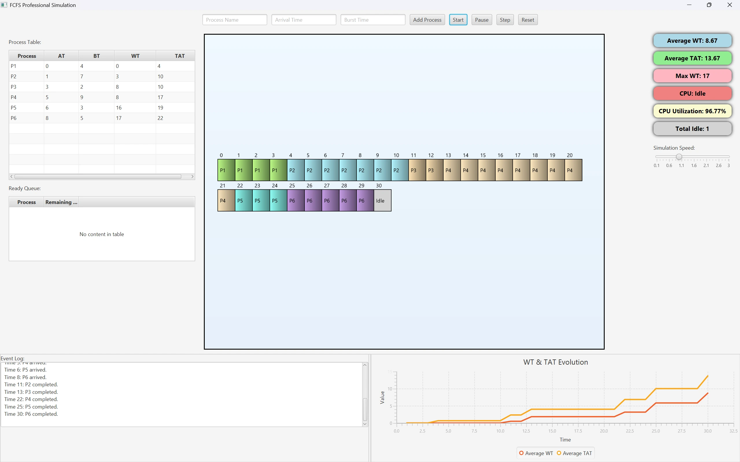
The application continuously computes performance metrics as the simulation timer runs. These parameters are essential for evaluating scheduling efficiency and understanding algorithm performance.
Waiting & Turnaround Time
Calculates waiting time (WT) and turnaround time (TAT) dynamically for each process. WT represents the total cycles a process spends in the ready queue, while TAT measures the duration from arrival to completion.
CPU Utilization & Idle Margin
Measures CPU efficiency. CPU Utilization tracks the percentage of execution cycles spent processing jobs, while Idle Time logs cycles when no processes are ready, identifying system bottlenecks.
Interactive Visualization
Mapping CPU execution cycles onto an active canvas.
Interactive visualization makes it easier to trace algorithm states. By rendering processes in real time, the application provides immediate visual context for queue management and CPU dispatch operations.
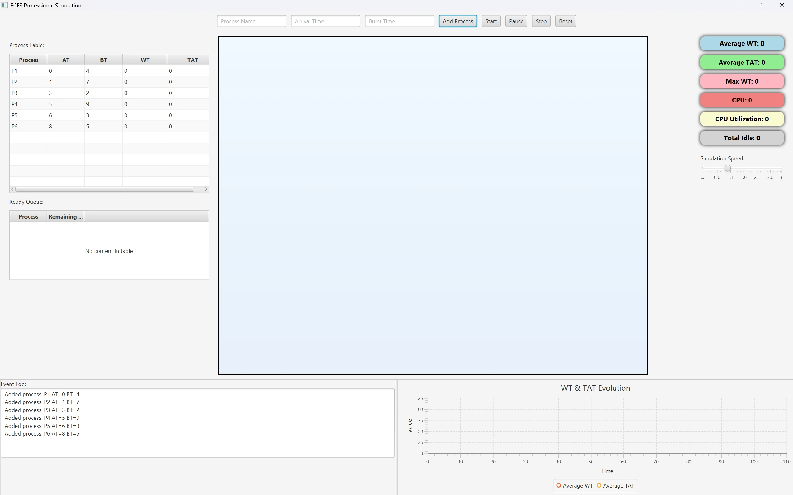
Updates dynamically, adding block segments as execution cycles progress, using colors to differentiate processes.
Resizes the rendering canvas automatically to display long execution sequences without clipping.
Shows process cards within the ready queue in real time, illustrating arrivals and order adjustments.
Engineering Highlights
Key implementation details of the desktop simulator.
Built as a JavaFX desktop tool for low-latency interface rendering.
Manages state updates through an asynchronous simulation loop.
Allows stepping through process execution cycle-by-cycle manually.
Computes turnaround, waiting, and utilization metrics automatically.
Renders process blocks on a canvas that resizes automatically.
Implements reactive controls to handle simulation state changes.
Presents process logs and final statistics in structured tables.
Decouples scheduling calculations from visual layout rendering.
Lessons Learned
Interactive simulators help students understand dynamic operating system concepts much better than static diagrams. Giving students control over the timer lets them observe scheduling operations at their own pace.
Decoupling the scheduling engine logic from the visual layout rendering simplifies development. The simulation engine manages pure queue states and statistics, which are then passed to the JavaFX scene graph for rendering.
Real-time analytics help students connect process arrivals and CPU activity directly to final waiting times and CPU utilization percentages, reinforcing the underlying scheduling mechanics.